Waffle charts are a great way to visualize data as a grid of squares where each square represents a portion of the whole. Unlike pie charts, which can be hard to interpret with many categories, waffle charts provide a cleaner, grid-based approach that makes it easy to compare parts of a dataset. They’re perfect for showing proportions, like market share, and provide a more visually appealing alternative to pie charts.

Although Excel doesn’t have a built-in waffle chart option, we can easily create one ourselves using conditional formatting and simple formulas. In this blog post, we’ll walk through building a waffle chart to visualize smartphone market share, using a small number of categories, making it an ideal choice.

Download the exercise file below to follow along:

Waffle choice 1: Visualizing one brand’s market share

Let’s begin by creating a chart that allows the user to select a brand and visualize its market share compared to the entire category. First, we’ll set up a simple 10×10 grid in the worksheet, which will proportionally represent the percentage breakdown of all the brands.

To create this grid, we can use the SEQUENCE() function to generate all integers from 1 to 100:

If it’s not entirely clear how this will come together yet, don’t worry—we’re just laying the groundwork. Next, we’ll set up a few fields where the user can choose which brand to focus on, along with a cell that will display the corresponding market share.

To enhance the user experience, you might consider adding a dropdown list using data validation, allowing the user to select the brand easily. I’ve included an example of this in the exercise file for you to explore. To retrieve the market share for the selected brand, we’ll use the XLOOKUP() function:

=XLOOKUP(B8, market_share[Brand], market_share[Market Share (%)])

Awesome work. Now, here’s where it gets interesting. I’ll set up an IF() statement in the workbook to compare the market share value to each cell in the 10×10 grid. If the grid value is less than or equal to the market share, the formula will flag it as a 1, otherwise, it will flag it as a 0. This will form the foundation for encoding the colors in the waffle chart, helping to visually represent the market share.

=IF(O3# <= B9, 1, 0)

Once you’ve set up the IF() statement, the next step is to visually encode the numbers using conditional formatting. Start by highlighting the range of cells in your 10×10 grid, then navigate to the Home tab and select Conditional Formatting. From there, choose Color Scales and click on More Rules. This will allow you to create a custom color palette for your waffle chart by assigning one color for cells flagged as 1 and another for cells flagged as 0.

From here, head down to the bottom of the rules and keep this a two-color scale but set up your own colors. I am going to use a lighter and darker shade of blue, this means the bigger the number the darker the shade, this will fill in our wafflechart with darker numbers for the market share each company has!

Awesome work! Your waffle chart should be coming together, but having the 1s and 0s still visible in the cells can be a bit distracting. Here’s how to clean that up:

To resolve this, select the range of cells where you want to hide the numbers, then press Ctrl + 1 on your keyboard to open the Format Cells menu. Navigate to the last option, Custom, and enter two or three semicolons (;;;). This trick will hide the data in the cells while keeping the formatting intact.

A couple more things to really polish this up: add some white borders between the cells to give it that classic waffle look! This will make the grid easier to read and visually appealing. Also, consider adding a dynamic chart title to make it more interactive. You can use a formula like this:

=CONCAT(B8, " has ", B9, "% market share")

This will automatically update the chart title based on the selected brand and its corresponding market share. At this point, you should have a nice, clean waffle chart.

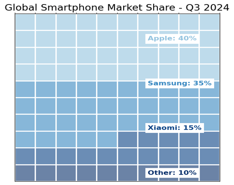
Waffle choice 2: Visualizing total market share by brand

Next, let’s work on creating a waffle chart that shows the total market share breakdown across all brands. We’ll use similar techniques, including the SEQUENCE(), IFS(), and conditional formatting functions, but this time we’ll need to add a few more layers of conditional logic.

To begin, let’s add a running total using structured table references. This will help us track cumulative market share for each brand. Use the following formula to calculate the running total:

=SUM(INDEX([Market Share (%)], 1):[@[Market Share (%)]])

This will sum the market share percentages from the first brand to the current brand, giving us a running total.

Now, using similar logic, I’ll create a 10×10 grid with conditional logic and formatting. The difference this time is that we’ll have multiple categories/colors, not just two. To achieve this, we’ll use the IFS() function to determine where each market share falls within the running total:

=IFS(R3# <= C2, 1,
R3# <= C3, 2,
R3# <= C4, 3,
R3# <= C5, 4)

The conditional formatting will work similarly, except this time, you’ll assign more colors—one for each category. I’ve already hidden the numbers, added the grids, and applied labels to clearly identify each brand.

This setup is a bit more labor-intensive and not as dynamic. If categories are added or removed from the data source, the chart can quickly go off track. Additionally, to prevent potential issues, we might want to add safeguards to ensure that the numbers in the data source sum to 100%. Let’s explore how we can handle that next.

Waffle choice 3: Dynamic wafflechart with Python in Excel

Lastly, I’d like to create a waffle chart that’s more dynamic and adaptable. I want to eliminate the need for all the manual steps like clicking, formatting, and adjusting, so the chart can automatically adjust to changes, such as a different number of categories or numbers that don’t sum to 100. For this, I’ll use Python code.

While it’s possible to create something similar in Excel using more dynamic formulas, I personally find Python much easier for tasks like this, especially with the help of tools like generative AI and Copilot. Of course, it’s all about what works best for you.

Here’s the Python code used to create this more dynamic waffle chart in Excel:

You should now have something like this:

As you’ll notice, the code is a bit extensive, so I won’t explain it all here. However, exploring websites like python-bloggers.com and embracing generative AI for questions can help you make significant progress with Python charts in Excel. Don’t hesitate to ask questions or experiment. You’ll see that the resulting plot will automatically adjust and resize as categories are added or removed, making it much more responsive and adaptable than the previous methods.

Conclusion

Although Excel doesn’t have a built-in waffle chart feature, you can easily create one with a few formulas and smart formatting (or by incorporating Python). It’s a sleek, visually appealing alternative to pie charts for comparing proportions, such as market share. This approach works best with a relatively small number of categories and provides a fresh perspective on presenting data. What questions do you have about creating waffle charts or data visualization in Excel? Let me know in the comments.

The post How to create a wafflechart in Excel first appeared on Stringfest Analytics.